Loan Default Prediction Project Using Machine Learning

For this project, we will be exploring publicly available data from Lending Club connects people who need money (borrowers) with people who have money (investors). Hopefully, as an investor, you would want to invest in people who showed a profile of having a high probability of paying you back. We will try to create a model that will help predict this.

We Solve this Project in 6 Phase

1. Business Understanding
2. Data Understanding
3. Data Preparation
4. Modeling
5. Evaluation
6. Deployment

1. Business Understanding

For this project, we will be exploring publicly available data from LendingClub.com. Lending Club connects people who need money (borrowers) with people who have money (investors). Hopefully, as an investor, you would want to invest in people who showed a profile of having a high probability of paying you back. We will try to create a model that will help predict this.

Lending Club is a US peer-to-peer lending company, headquartered in San Francisco, California. It was the first peer-to-peer lender to register its offerings as securities with the Securities and Exchange Commission (SEC) and to offer loan trading on a secondary market. Lending Club operates an online lending platform that enables borrowers to obtain a loan, and investors to purchase notes backed by payments made on loans. Lending Club is the world's largest peer-to-peer lending platform. Lending Club enables borrowers to create unsecured personal loans between 1,000and1,000and40,000. The standard loan period is three years. Investors can search and browse the loan listings on the Lending Club website and select loans that they want to invest in based on the information supplied about the borrower, amount of loan, loan grade, and loan purpose. Investors make money from interest. Lending Club makes money by charging borrowers an origination fee and investors a service fee.

Problem Statement: To classify if the borrower will default the loan using the borrower’s financial history. That means, given a set of new predictor variables, we need to predict the target variable as 1 -> Defaulter or 0 -> Non-Defaulter. The metric we use to choose the best model is ‘False Negative Rate’. (predictor and target variables explained later)

Import Nessecerry Libraries

import pandas as pd 
import matplotlib.pyplot as plt 
import seaborn as sns 
%matplotlib inline 
import warnings    #remove warning messege in our project file 
warnings.filterwarnings('ignore')3,2,1] 
 'home_ownership' = ['MORTGAGE', 'OWN', 'RENT', 'NONE', 'OTHER', 'ANY'] to [6,5,4,3,2,1] 
 'emp_length' = ['3 years', '10+ years', '5 years', '4 years', '6 years', '1 year','2 years', '7 years', '9 years', '8 years', '< 1 year', 'n/a'] to [int], remove string 
 values , n/a and change type to int 
 'int_rate' = remove % sign and change to int 
from IPython.core.display import HTML    #for good look display we import html display 
from sklearn.preprocessing import StandardScaler   #Convert data into Standard Scale 
from sklearn.model_selection import train_test_split     #for split data into tranning dataset and testing dataset 
from sklearn.feature_selection import RFE     #Feature selection using Recursive Feature Elimination 
from sklearn.linear_model import LogisticRegression   #Logistic Regresssion Algrothim 
from sklearn.ensemble import RandomForestClassifier  #Random Forest Classifer Algrothim 
from sklearn.metrics import confusion_matrix,classification_report  #for Confussion matrix and classification report 
from sklearn.tree import DecisionTreeClassifier   #Decision Tree Classifier Algrothims 
from sklearn.neighbors import KNeighborsClassifier   #KNN(K Near Neghbors Algrothims) 

2. Data Understanding Phase Start.

#first data set
loan_2012_2013 = pd.read_csv("2012-2013.csv")
#second data set
loan_2014 = pd.read_csv('2014loan.csv')
#Check the type of data set.
print(type(loan_2012_2013),type(loan_2014))
#Check the shape of data set.
print((loan_2012_2013).shape,(loan_2014).shape)

Check First Data Set and Collect Information About it

#check Head of our Data frame
loan_2012_2013.head(5)
loan_2012_2013.describe(include='all')

Check Missing Values in Our first Data set

#check missing values in first data set
print(loan_2012_2013.isnull().sum())
print('Rows in Data set', loan_2012_2013.shape[0],'Columns in Data set ', loan_2012_2013.shape[1])

Check Second Data set

loan_2014.head()
loan_2014.info()
loan_2014.describe()

check Missing Values in Second Data Set

loan_2014.isnull().sum()
loan_2014.info()

3. Data Prepration

Concatenation Above Two DataSet and Create a New DataFrame is Called loandataset

loandataset = pd.concat([loan_2012_2013, loan_2014])
loandataset.head()

Now Check Shape of loandataset

print('Rows in Data set', loandataset.shape[0],'Columns in Data set ', loandataset.shape[1])

Missing value Treatment

loandataset.isnull().sum()

Now Drop Empty Columns in loandataset

loandatasetnew=loandataset.dropna(axis=1,thresh=len(loandataset)*0.9) 
loandatasetnew.shape
loandataset = loandatasetnew

Check Head Again of loandataset

loandataset.head()
loandataset['purpose'].unique()

What is Target Column in loandataset ?

‘loan_status’

loandataset['loan_status'].head(10)
loandataset['loan_status'].unique()

Here are 8 Type of Unique Values but we target only two type of values

'Fully Paid' 'Charged off' We Convert Our Column values into 'Fully Paid' == 0 'Charged off' == 1 and create a new dataset is called Dataset_withBoolTarget

data_with_loanstatus_sliced = loandataset[(loandataset['loan_status']=="Fully Paid") | (loandataset['loan_status']=="Charged Off")]
di = {"Fully Paid":0, "Charged Off":1}   #converting target variable to boolean
Dataset_withBoolTarget= data_with_loanstatus_sliced.replace({"loan_status": di})
Dataset_withBoolTarget['loan_status'].head(10)

Now Count How many Number of fully paid and charged off values

print(Dataset_withBoolTarget['loan_status'].value_counts())
print('\n')
print("Current shape of dataset :",Dataset_withBoolTarget.shape)
Dataset_withBoolTarget.head(3)

Here We Drop Some More Unrelvent Values in DataSet

s=Dataset_withBoolTarget_corr.loc['loan_status',:]
list_week_relation_pos=s[(s <0.1) & (s> 0)] 
list_week_relation_neg=s[(s > -0.1) & (s < 0)]  
list_ps=list(list_week_relation_pos.index)
list_ng=list(list_week_relation_neg.index)
list_column_to_drop=list_ps+list_ng
print(len(list_column_to_drop))
#Dataset_withBoolTarget.drop(list_column_to_drop,axis=1,inplace=True)
print(Dataset_withBoolTarget.shape)
print(Dataset_withBoolTarget.head(5))

Here we Create our Final DataFrame is called 'Final_data'

features = ['int_rate','grade','emp_length','home_ownership','loan_status','out_prncp','out_prncp_inv','total_pymnt','total_pymnt_inv','total_rec_prncp','total_rec_late_fee','recoveries','collection_recovery_fee','last_pymnt_amnt','purpose'] 
Final_data = Dataset_withBoolTarget[features] #19 features with target var
Final_data.head(10)

Data Transformation

Here we do some transformation in 4 Columns of Object Type How we transformation in these columns ?

1. 'grade' = ['A', 'B', 'D', 'C', 'E', 'F', 'G'] to [7,6,5,4,3,2,1]
2. 'home_ownership' = ['MORTGAGE', 'OWN', 'RENT', 'NONE', 'OTHER', 'ANY'] to [6,5,4,3,2,1]
3. 'emp_length' = ['3 years', '10+ years', '5 years', '4 years', '6 years', '1 year','2 years', '7 years', '9 years', '8 years', '< 1 year', 'n/a'] to [int], remove string
4. values , n/a and change type to int
5. 'int_rate' = remove % sign and change to int

#Data encoding
Final_data['grade'] = Final_data['grade'].map({'A':7,'B':6,'C':5,'D':4,'E':3,'F':2,'G':1})
Final_data["home_ownership"] = Final_data["home_ownership"].map({"MORTGAGE":6,"RENT":5,"OWN":4,"OTHER":3,"NONE":2,"ANY":1})
Final_data["emp_length"] = Final_data["emp_length"].replace({'years':'','year':'',' ':'','<':'','\+':'','n/a':'0'}, regex = True)
#Final_data["emp_length"] = Final_data["emp_length"].apply(lambda x:int(x))
print("Current shape of dataset :",Final_data.shape)
Final_data.head()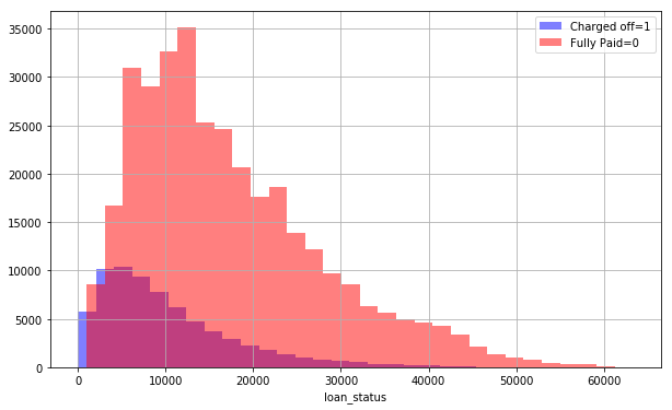

Exploratory Data Analysis

Check Numbers of Fully Paid and Charged off Customers

Here We Check Purpose of Loan By Visualization Graph

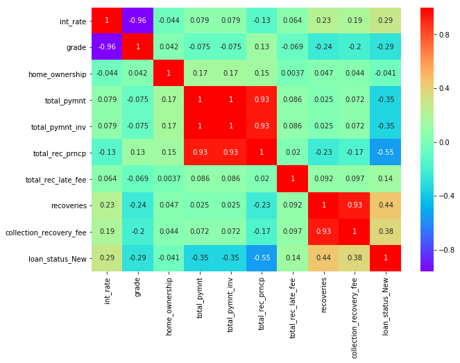
Correlation Between all column to each other

4. Model Creation

Train test split

from sklearn.model_selection import train_test_split
data_clean.head()
#print(data_clean.isnull().sum())
data_clean['loan_status_New']=data_clean['loan_status']
data_clean.head(2)
data_clean.drop('loan_status',axis=1,inplace=True)

Now we create a two different variable First X variable hold all column without target and y varable hold our target column

X = data_clean.iloc[:,:-1]
y = data_clean.iloc[:,-1]
X_train, X_test, y_train, y_test = train_test_split(X, y, test_size=0.3, random_state=101)

Evalulate Different Models and Find Best Accuracy in Models

Here is a List of Differnet type of Algrothims we use

1. Random Forest Classifer
2. Decision Tree
3. Logistic Regression Classifer
4. K Near Neighbors 
    

Train DataSet Using Random Forest model

from sklearn.ensemble import RandomForestClassifier
rfc = RandomForestClassifier(n_estimators=600)  #create instance
rfc.fit(X_train,y_train)

Evaluation of Random Forest Model

prediction = rfc.predict(X_test)
from sklearn.metrics import confusion_matrix,classification_report,accuracy_score
print(rfc_report)
print(confusion_matrix(y_test,prediction))
print(accuracy_score(y_test, prediction, normalize=True))

All Algrothims Used in Jupyter Notebook Download Notebook for this Project and Get Complete Information of this Project

Here we Check Classification Report for all above Models and Check Who's Model Give us Best Accuracy Score.

print("________________Random Forest Classification Report__________________\n")
print('RFC',rfc_report)
print('**********************************************************************\n')
print("________________Decision Tree Classification Report__________________\n")
print('DTree',dtree_report)
print('**********************************************************************\n')
print("________________Logistic Regression Classification Report__________________\n")
print('llogtt',lreport)
print('**********************************************************************\n')
print("________________K Nearest Neighbor Classification Report__________________\n")
print('knnreport',knnreport)

Conclusion

We Check all of these Model Result and than we getb Random Forest Model have a Best Accuracy other than and it's also have a Better Classification Report. So,We can say that 'The random forest model is best for our dataset'.

Download Jupyter Notebook  

Thanks for Reading  
Share this Project With Your Network