Time Series Analysis on Air Passenger Data

Time series analysis is crucial for understanding trends, seasonality, and making future predictions based on historical data. In this blog, we will analyze the famous AirPassengers dataset, perform decomposition, check for stationarity, build an ARIMA model for forecasting, and detect anomalies.

Goal

Our goal is to analyze the AirPassengers dataset to:

1. Identify trends and seasonal patterns.
2. Check stationarity of the dataset.
3. Build an ARIMA model for forecasting.
4. Detect anomalies in the data.

Required Packages

Before we start, install the necessary Python packages:

pip install pandas matplotlib statsmodels numpy

Step 1: Load and Inspect the Data

We first load the dataset and inspect its structure.

import pandas as pd  
import matplotlib.pyplot as plt  
from statsmodels.tsa.seasonal import seasonal_decompose  
import numpy as np  
from statsmodels.tsa.stattools import adfuller  
from statsmodels.tsa.arima.model import ARIMA  
# Load dataset
df = pd.read_csv("AirPassengers.csv", parse_dates=["Month"], index_col="Month")  
# Display first few rows
print(df.head())  
print(df.info()) 

Step 2: Data Visualization

Plot the data to understand trends and seasonality.

plt.figure(figsize=(12,6))  
plt.plot(df.index, df["#Passengers"], label="Monthly Passengers")  
plt.xlabel("Year")  
plt.ylabel("Passengers (in thousands)")  
plt.title("Air Passenger Traffic Over Time")  
plt.legend()  
plt.show()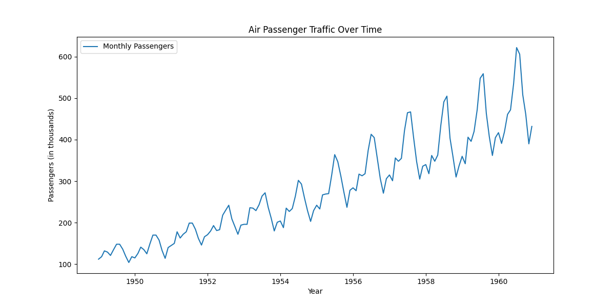 

Step 3: Handle Missing Values

print(df.isnull().sum())  # Check for missing values
df = df.fillna(method="ffill")  # Forward fill if necessary

Step 4: Decomposing the Time Series

We decompose the time series into trend, seasonal, and residual components.

# Decomposing the time series  
decomposed = seasonal_decompose(df["#Passengers"], model="multiplicative", period=12)  
# Plot the decomposition
decomposed.plot()  
plt.show()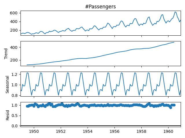  

Step 5: Test for Stationarity (ADF Test)

We use the Augmented Dickey-Fuller test to check stationarity.

result = adfuller(df["#Passengers"])  
print(f"ADF Statistic: {result[0]}")  
print(f"P-value: {result[1]}")  

If the p-value is greater than 0.05, the data is non-stationary.

To make the series stationary, we apply differencing:

df["Passengers_diff"] = df["#Passengers"].diff().dropna()  
# Re-run ADF test
result = adfuller(df["Passengers_diff"].dropna())  
print(f"New ADF Statistic: {result[0]}")  
print(f"New P-value: {result[1]}")  

Step 6: Train-Test Split

train_size = int(len(df) * 0.8)  
train, test = df.iloc[:train_size], df.iloc[train_size:]  

Step 7: Train an ARIMA Model

# Train ARIMA Model
model = ARIMA(train["#Passengers"], order=(1,1,1))  
model_fit = model.fit()  
# Forecast
forecast = model_fit.forecast(steps=len(test))  
# Plot results
plt.plot(test.index, test["#Passengers"], label="Actual")  
plt.plot(test.index, forecast, label="Forecast", linestyle="dashed")  
plt.legend()  
plt.show() 

Step 8: Detecting Anomalies using Z-Score

df["Z-Score"] = (df["#Passengers"] - df["#Passengers"].mean()) / df["#Passengers"].std()  
df["Anomaly"] = df["Z-Score"].abs() > 3  # Mark anomalies if Z-score > 3  
# Plot anomalies
plt.plot(df.index, df["#Passengers"], label="#Passengers")  
plt.scatter(df.index[df["Anomaly"]], df["#Passengers"][df["Anomaly"]], color="red", label="Anomalies")  
plt.legend()  
plt.show()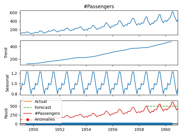 

Conclusion

In this analysis, we:

• Visualized the data to identify trends and seasonality.
• Checked for stationarity and made adjustments.
• Built an ARIMA model for forecasting future values.
• Detected anomalies using Z-Score. This approach can be applied to any time series dataset to gain insights and make informed decisions.

Download Dataset

Full Code

import pandas as pd  
import matplotlib.pyplot as plt  
from statsmodels.tsa.seasonal import seasonal_decompose  
import numpy as np  
from statsmodels.tsa.stattools import adfuller  
from statsmodels.tsa.arima.model import ARIMA  
# Load dataset
df = pd.read_csv("AirPassengers.csv", parse_dates=["Month"], index_col="Month")  
# Handle missing values
df = df.fillna(method="ffill")  
# Visualization
plt.figure(figsize=(12,6))  
plt.plot(df.index, df["#Passengers"], label="Monthly Passengers")  
plt.xlabel("Year")  
plt.ylabel("Passengers (in thousands)")  
plt.title("Air Passenger Traffic Over Time")  
plt.legend()  
plt.show()  
# Decomposing the time series  
decomposed = seasonal_decompose(df["#Passengers"], model="multiplicative", period=12)  
decomposed.plot()  
plt.show()  
# ADF Test
result = adfuller(df["#Passengers"])  
print(f"ADF Statistic: {result[0]}")  
print(f"P-value: {result[1]}")  
# Differencing
df["Passengers_diff"] = df["#Passengers"].diff().dropna()  
result = adfuller(df["Passengers_diff"].dropna())  
print(f"New ADF Statistic: {result[0]}")  
print(f"New P-value: {result[1]}")  
# Train-Test Split
train_size = int(len(df) * 0.8)  
train, test = df.iloc[:train_size], df.iloc[train_size:]  
# Train ARIMA Model
model = ARIMA(train["#Passengers"], order=(1,1,1))  
model_fit = model.fit()  
forecast = model_fit.forecast(steps=len(test))  
plt.plot(test.index, test["#Passengers"], label="Actual")  
plt.plot(test.index, forecast, label="Forecast", linestyle="dashed")  
plt.legend()  
plt.show()  
# Detect Anomalies
df["Z-Score"] = (df["#Passengers"] - df["#Passengers"].mean()) / df["#Passengers"].std()  
df["Anomaly"] = df["Z-Score"].abs() > 3  
plt.plot(df.index, df["#Passengers"], label="#Passengers")  
plt.scatter(df.index[df["Anomaly"]], df["#Passengers"][df["Anomaly"]], color="red", label="Anomalies")  
plt.legend()  
plt.show()