Window Functions in SQL – The Ultimate Guide

Window functions are one of the most powerful tools in SQL. They allow you to perform calculations across rows that are related to the current row without collapsing the result set like GROUP BY does. This makes them ideal for ranking, running totals, moving averages, and other analytics tasks.

This guide will break down the components of window functions, explain how they work, and walk through the most commonly used window functions with real-world examples.

What is a Window Function?

A window function performs a calculation across a set of table rows that are somehow related to the current row. Unlike aggregate functions, window functions do not group the rows into a single output row — they return a value for each row.

Basic Syntax

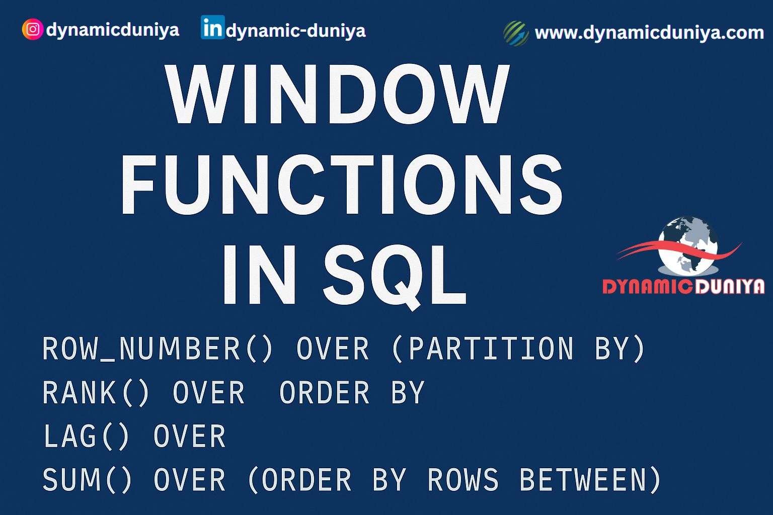
function_name() OVER (
    PARTITION BY column_name
    ORDER BY column_name
    ROWS BETWEEN ...
)

Components of a Window Function

1. Function Name: E.g., ROW_NUMBER(), SUM(), AVG(), RANK(), etc.
2. OVER() clause: Defines the "window" (i.e., subset of rows) the function should operate on.
3. PARTITION BY: (Optional) Divides the result set into partitions to apply the function separately.
4. ORDER BY: (Optional but common) Defines the order of rows within each partition.
5. ROWS BETWEEN: (Optional) Limits the window frame (used mostly in cumulative or moving aggregates).

Common and Most Useful SQL Window Functions

1. ROW_NUMBER()

Assigns a unique sequential integer to rows within a partition.

Example:

SELECT employee_id, department, salary,
       ROW_NUMBER() OVER (PARTITION BY department ORDER BY salary DESC) AS rank_in_dept
FROM employees;

Use Case: Ranking employees in each department based on salary.

2. RANK() and DENSE_RANK()

RANK() skips numbers in case of ties.

DENSE_RANK() does not skip numbers for ties.

Example:

SELECT employee_id, department, salary,
       RANK() OVER (PARTITION BY department ORDER BY salary DESC) AS salary_rank
FROM employees;

Use Case: Identify top earners in each department, even if some have the same salary.

3. NTILE(n)

Distributes rows into n approximately equal buckets.

Example:

SELECT student_id, marks,
       NTILE(4) OVER (ORDER BY marks DESC) AS quartile
FROM students;

Use Case: Splitting students into quartiles based on performance.

4. LAG() and LEAD()

• LAG() returns the previous row’s value.
• LEAD() returns the next row’s value.

Example:

SELECT product_id, sale_date, sales,
       LAG(sales, 1, 0) OVER (PARTITION BY product_id ORDER BY sale_date) AS previous_sales,
       LEAD(sales, 1, 0) OVER (PARTITION BY product_id ORDER BY sale_date) AS next_sales
FROM sales_data;

Use Case: Comparing current sales to previous and next periods.

5. SUM(), AVG(), MIN(), MAX() as Window Functions

Same as aggregate functions but used without collapsing rows.

Example (Running Total):

SELECT order_id, customer_id, order_value,
       SUM(order_value) OVER (PARTITION BY customer_id ORDER BY order_date) AS running_total
FROM orders;

Use Case: Running totals of customer orders.

Window Frame (ROWS BETWEEN clause)

By default, most aggregate window functions operate on RANGE BETWEEN UNBOUNDED PRECEDING AND CURRENT ROW. But we can control the window frame precisely:

Example (Moving Average over 3 rows):

SELECT order_date, order_value,
       AVG(order_value) OVER (
         ORDER BY order_date
         ROWS BETWEEN 2 PRECEDING AND CURRENT ROW
       ) AS moving_avg
FROM orders;

Use Case: 3-day moving average of sales.

Common Options for ROWS BETWEEN

1. UNBOUNDED PRECEDING – From the first row in the partition
2. CURRENT ROW – The current row
3. n PRECEDING – n rows before the current row
4. n FOLLOWING – n rows after the current row
5. UNBOUNDED FOLLOWING – Up to the last row in the partition

Examples

• Cumulative Sum:

SUM(amount) OVER (ORDER BY date ROWS BETWEEN UNBOUNDED PRECEDING AND CURRENT ROW)

• Centered Moving Average (2 before, 2 after):

AVG(sales) OVER (ORDER BY date ROWS BETWEEN 2 PRECEDING AND 2 FOLLOWING)

• Future Sum Only:

SUM(sales) OVER (ORDER BY date ROWS BETWEEN CURRENT ROW AND UNBOUNDED FOLLOWING)

These options provide precise control over the window for each calculation.

Real-World Use Cases

1. Customer Purchase Trends

SELECT customer_id, purchase_date, amount,
       SUM(amount) OVER (PARTITION BY customer_id ORDER BY purchase_date) AS cumulative_spend
FROM purchases;

2. Employee Attrition Tracking

SELECT employee_id, join_date, exit_date,
       LEAD(join_date) OVER (PARTITION BY department ORDER BY join_date) AS next_joined_employee
FROM employee_records;

3. Stock Price Change Detection

SELECT stock_id, date, closing_price,
       closing_price - LAG(closing_price) OVER (PARTITION BY stock_id ORDER BY date) AS price_change
FROM stock_prices;

Best Practices

• Use PARTITION BY wisely — too many partitions can reduce performance.
• Always use ORDER BY in window functions where sequence matters.
• Test window frame behavior with ROWS BETWEEN to get precise control over calculations.
• Use indexes on columns used in PARTITION BY and ORDER BY for performance tuning.

Conclusion

SQL Window Functions are essential for modern analytics and reporting tasks. They empower developers and data professionals to write cleaner, more efficient, and highly expressive queries. Mastering these functions can significantly improve the way you handle complex data manipulations in SQL.

Whether you’re doing time-series analysis, rankings, or rolling aggregates — window functions make it easier, cleaner, and faster.